Exercise: Thermal conductivity of CuI from aiGK#
In this exercise, you will:
- Perform ab initio Green Kubo calculations
- Learn the simulation time convergence of Green-Kubo method
- Estimate anharmonicity change of CuI
Using Green-Kubo theory in combination with ab initio molecular dynamics simulations, we can calculate the thermal conductivity including full anharmonicity. To calculate the Green-Kubo formula from first principles, the energy \(E^{\rm DFT}(\boldsymbol{R})\), forces \(\boldsymbol{F}(\boldsymbol{R})\), stress tensor \(\boldsymbol{\sigma}(\boldsymbol{R})\) and atomic contribution of stress tensor \(\boldsymbol{\sigma}_{I}(\boldsymbol{R})\) must be calculated, and we do that in this tutorial with FHI-aims.
Setting up ab initio MD#
We will use a 216 atom supercell of CuI and the PBEsol functional for this MD simulation. The following geometry files needs to be prepared,
geometry.in.primitive: primitive cell from relaxation
geometry.in.supercell: supercell at equilibrium
geometry.in: thermalized supercell as the initial step of MD
Note that geometry.in is obtained from a MD trajectory in NVT ensemble,
This will be introduced in Ensemble average.
Examples can be found in the input directory.
Prepare md.in#
In md.in file, we need to specify settings for both first principle calculations
and the MD calculation.
Settings for the first principle calculation#
[calculator]
name:                          aims
socketio:                      true

[calculator.parameters]
xc:                            pbesol
compute_forces:                true
compute_analytical_stress:     true

[calculator.kpoints]
density:                       2

[calculator.basissets]
Cu:                            light
I:                             light
Here we are using a aims calculator, with the PBEsol functional, k-point density of 2
and light species defaults for all atoms. The calculation of forces and analytical stresses
are enabled for the MD simulation and virial heat flux calculation.
Settings for MD simulation#
[md]
driver:                        VelocityVerlet
timestep:                      5
maxsteps:                      12000
compute_stresses:              2
workdir:                       md

[md.kwargs]
logfile:                       md.log

[files]
geometry:                      geometry.in
primitive:                     geometry.in.primitive
supercell:                     geometry.in.supercell

[restart]
command:                       sbatch submit.sh
For the Green Kubo calculation, the time correlation function is calculated from a
microcanonical ensemble, namely, the NVE ensemble. Here we use the Verlet algorithm for
updating the velocity. The simulation time step is set to be 5 fs, and
the maxsteps is set to 12000 steps corresponding to 60 ps. To speed up the
calculation, the stresses calculation is calculated every 2 steps.
MD simulations can takes a days or even weeks to months to run. By using [restart] setting in md.in,
the job can be restarted if you run into wall-time limits on your HPC resources.
Settings for submission to HPC resources#
An example of a user prepared submit script to HPC resources using SLURM is given here:
Example for the submission script on the webinar cluster submit.sh
#!/bin/bash -l
# Standard output and error:
#SBATCH -o ./slurm.stdout
#SBATCH -e ./slurm.stderr
# Initial working directory:
# Standard output and error:
#SBATCH -o ./slurm.stdout
#SBATCH -e ./slurm.stderr
# Initial working directory:
#SBATCH -D ./
# Job Name:
#SBATCH -J FHI-aims
# Number of nodes and MPI tasks per node:
#SBATCH --nodes=1
# HPC7a
#SBATCH --tasks-per-node=192
#
# Wall clock limit:
#SBATCH --time=10:00:00

module purge
module load fhi-aims vibes

vibes run md
The calculation can be submitted through this command:
Settings for submission in vibes input file (optional)#
Alternatively, a submit script can also be generated by FHI-vibes template
with the following settings in the input file md.in
[slurm]
name:                          aigk
tag:                           vibes
mail_type:                     none
mail_address:                  your@mail.com
nodes:                         2
cores:                         96
queue:                         general
timeout:                       600
The setting allows you submit the calculation using command vibes submit md.
Results#
During the simulation, we can use the following command to output results,
This command will generate an NetCDF file trajectory.nc and a json-type output file
trajectory.son with all the essential information from the MD trajectory.
To read this file, you can use the following command
Output of vibes info md trajectory.nc
Dataset summary for trajectory.nc:

[info]         Summarize Displacements
Avg. Displacement:             0.22949 AA
Max. Displacement:             2.8811 AA
Avg. Displacement [Cu]:        0.26255 AA
Avg. Displacement [I]:         0.19642 AA

[info]         Summarize Forces
Avg. Force:                    1.1855e-19 eV/AA
Std. Force:                    0.35737 eV/AA
Std. Force [Cu]:               0.30548 eV/AA
Std. Force [I]:                0.40264 eV/AA

[info]         Summarize Temperature
Simulation time:                 60.000 ps (12001 steps)
Temperature:                       310.237 +/-      12.7020 K
Temperature (first 1/2):           311.385 +/-      12.4513 K
Temperature (last  1/2):           309.089 +/-      12.8466 K
Temperature drift:                  -0.05838 K/ps

[info]         Summarize Potential Pressure
Simulation time:                 60.000 ps (3062 of 12001 steps)
Pressure:                          0.061724 +/-   0.056299 GPa
Pressure (last 1/2):               0.046461 +/-   0.055929 GPa
Pressure (last 1/2):               0.000290 +/-   0.000349 eV/AA**3
[info]         Summarize Total Pressure (Kinetic + Potential)
Simulation time:                 60.000 ps (3062 of 12001 steps)
Pressure:                          0.219238 +/-   0.054823 GPa
Pressure (last 1/2):               0.203353 +/-   0.054621 GPa
Pressure (last 1/2):               0.001269 +/-   0.000341 eV/AA**3

[info]         Drift
Mean abs. Momentum:            [1.8597e-13 1.6907e-13 1.5333e-13] AA/fs
Energy drift:                  -1.02111e-05  eV / timestep
Energy change after 100ps:     -2.04222e-01  eV
Energy change after 100ps:     -9.45472e-01  meV / atom (n=216)
You can verify that the calculation has run correctly by e.g. checking the temperature is what was targeted, and making sure that the energy drift it small. One call also see from the maximum displacement of 2.88 AA during the simulation that this is a strongly anharmonic system.
As running ab initio MD in extended supercells for tens of picoseconds takes considerable computer time, you can also analyse pre-calculated trajectories from Ref. 1, from here (nve.1 ~1 GB filesize).
Obtaining the pre-calculated trajectory
The pre-calculated trajectory is currently stored in the vibes-tutorial-files repository. To obtain it, one needs to clone the repo and checkout the branch:
The trajectory filetrajectory.nc in the directory 7_green_kubo/nve.1, is stored in Git Large File Storage due to it's large size. To access it, one needs to download and install the
git lfs command line extension from here. Then, the complete file can be obtained with the following commands:
Postprocess#
After we obtained the file trajectory.nc,
we use the following command,
You will get the following information from the output,
Run aiGK output workflows for trajectory.nc
[GreenKubo]    Compute Prefactor:
[GreenKubo]    .. Volume:           5873.07  AA^3
[GreenKubo]    .. Temperature:       310.24  K
[GreenKubo]    -> Prefactor:      1.135e+03  W/mK / (eV/AA^2/fs)
[GreenKubo]    Estimate filter window size
[GreenKubo]    .. lowest vibrational frequency: 0.8364 THz
[GreenKubo]    .. corresponding window size:    1195.5435 fs
[GreenKubo]    .. window multiplicator used:    1.0000 fs
[filter]       Apply Savitzky-Golay filter with {'window_length': 61, 'polyorder': 1}
[GreenKubo]    Cutoff times (fs):
[GreenKubo]    [[5360.    0.    0.]
[GreenKubo]     [   0. 1480.  940.]
[GreenKubo]     [   0.  420. 2960.]]
[GreenKubo]    Kappa is:       0.795 +/- 0.274 W/mK
[GreenKubo]    Kappa^ab is:
[GreenKubo]    [[ 1.423e+00 -1.168e-03 -1.080e-03]
[GreenKubo]     [-1.387e-04  2.769e-01  1.053e-02]
[GreenKubo]     [-1.092e-03  1.441e-02  6.843e-01]]
The thermal conductivity tensor is calculated by the integration of the time correlation function of the heat flux.
We can also visualise the heat flux auto-correlation function and the thermal conductivity with the following command
which will produce a file calledgreenkubo_summary.pdf which is shown below.
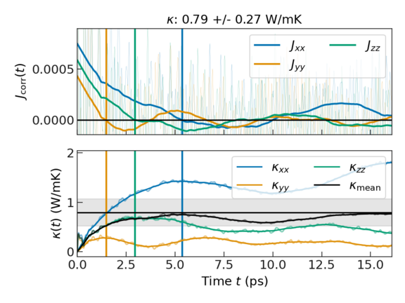
The upper plot shows the heat flux auto-correlation function. The thin lines show the raw data, while the thick lines show the post-processed data, for which the noise and fluctuations that do not contribute to the thermal conductivity have been removed. The vertical lines indicate the earliest occurrence of the auto-correlation functions crossing the x-axis. We assume that the auto-correlation function is trustworthy up to this "first dip". Accordingly, the thermal conductivities reported in the output are obtained by integrating up to this time.
The lower plot shows the running integral of the above auto-correlation functions that yields the thermal conductivity. Each colored line represents a different direction (xx, yy, zz), the black line their mean, and the shaded area the associated standard deviation.
CuI is cubic system showing space group \(\rm F\bar{4}3m\), following Neumann’s principle, the symmetry operation reduces the thermal conductivity tensor to independent coefficients with \(\kappa_{xx} = \kappa_{yy} = \kappa_{zz}\). The error of the three components shown in the plot arises from thermal fluctuations and statistical error.
Finite-size correction#
Limited by the computational cost, we can only calculate ab initio molecular dynamics
from a finite supercell, thus, phonon wavelengths greater than the cell size
are missing in our calculation. Therefore, we need a finite-size correction to include
those long wavelength phonon modes, especially acoustic modes.
The theory of the finite-size correction is introduced in
2 and 1, and the method is
implemented in FHI-vibes.
A harmonic phonon model is used in the finite-size correction. We will use the harmonic force constants
we obtained in Exercise 1: Phonon dispersion, and
calculate the harmonic properties from these previously calculated force constants, (available in the file
FORCE_CONSTANTS from phonopy).
We then append the harmonic properties and force constants to the trajectory.nc file with the following command:
If you are using the pre-calculated trajectory.nc files, the force constants and harmonic properties are already included, so
there is no need to do the above command. You can just continue with the following steps.
The finite-size extrapolation can be easily calculated with the following command:
You will get the following output detailing what the interpolation is doing
Output of vibes output gk --interpolate --plot trajectory.nc
Run aiGK output workflows for trajectory.nc
[GreenKubo]    Compute Prefactor:
[GreenKubo]    .. Volume:           5873.07  AA^3
[GreenKubo]    .. Temperature:       310.24  K
[GreenKubo]    -> Prefactor:      1.135e+03  W/mK / (eV/AA^2/fs)
[GreenKubo]    Estimate filter window size
[GreenKubo]    .. lowest vibrational frequency: 0.8364 THz
[GreenKubo]    .. corresponding window size:    1195.5435 fs
[GreenKubo]    .. window multiplicator used:    1.0000 fs
[filter]       Apply Savitzky-Golay filter with {'window_length': 61, 'polyorder': 1}
[GreenKubo]    Cutoff times (fs):
[GreenKubo]    [[5360.    0.    0.]
[GreenKubo]     [   0. 1480.  940.]
[GreenKubo]     [   0.  420. 2960.]]
[GreenKubo]    Kappa is:       0.795 +/- 0.274 W/mK
[GreenKubo]    Kappa^ab is:
[GreenKubo]    [[ 1.423e+00 -1.168e-03 -1.080e-03]
[GreenKubo]     [-1.387e-04  2.769e-01  1.053e-02]
[GreenKubo]     [-1.092e-03  1.441e-02  6.843e-01]]
[lattice_points] .. matched 216 positions in supercell and primitive cell in 0.925s
[symmetry]     reduce q-grid w/ 108 points
[symmetry]        |||||||||||||||||||||||||||||||||||||  108/108
[symmetry]     .. q-points reduced from 108 to 24 points. in 0.053s
[force_constants] remap force constants
[force_constants] .. time elapsed: 0.531s
[force_constants] ** Force constants are not symmetric by 1.34e-02.
[force_constants] -> Symmetrize force constants.
[force_constants] ** Sum rule violated by 1.29e-02 (axis 1).
[dynamical_matrix] Setup complete, eigensolution is unitary.
[gk.harmonic]  Get lifetimes by fitting to exponential
[gk.harmonic]  ** acf drops fast for s, q: 0, 0 set tau_sq = np.nan
[gk.harmonic]  ** acf drops fast for s, q: 1, 0 set tau_sq = np.nan
[gk.harmonic]  ** acf drops fast for s, q: 2, 0 set tau_sq = np.nan
[gk.harmonic]  .. time elapsed: 0.678s
[gk.interpolation] Interpolated l_sq at Gamma: [21.07 46.7  39.68 17.55 10.65 15.17]
[symmetry]     reduce q-grid w/ 64 points
[symmetry]        |||||||||||||||||||||||||||||||||||||  64/64
[symmetry]     .. q-points reduced from 64 to 19 points. in 0.084s
[gk.interpolation]   4, Nq_eff =   0.59, kappa = 0.580 W/mK
[symmetry]     reduce q-grid w/ 216 points
[symmetry]        |||||||||||||||||||||||||||||||||||||  216/216
[symmetry]     .. q-points reduced from 216 to 52 points. in 0.033s
[gk.interpolation]   6, Nq_eff =   2.00, kappa = 0.997 W/mK
[symmetry]     reduce q-grid w/ 512 points
[symmetry]        |||||||||||||||||||||||||||||||||||||  512/512
[symmetry]     .. q-points reduced from 512 to 112 points. in 0.053s
[gk.interpolation]   8, Nq_eff =   4.74, kappa = 1.225 W/mK
[symmetry]     reduce q-grid w/ 1000 points
[symmetry]        |||||||||||||||||||||||||||||||||||||  1000/1000
[symmetry]     .. q-points reduced from 1000 to 206 points. in 0.100s
[gk.interpolation]  10, Nq_eff =   9.26, kappa = 1.346 W/mK
[symmetry]     reduce q-grid w/ 1728 points
[symmetry]        |||||||||||||||||||||||||||||||||||||  1728/1728
[symmetry]     .. q-points reduced from 1728 to 343 points. in 0.219s
[gk.interpolation]  12, Nq_eff =  16.00, kappa = 1.423 W/mK
[symmetry]     reduce q-grid w/ 2744 points
[symmetry]        |||||||||||||||||||||||||||||||||||||  2744/2744
[symmetry]     .. q-points reduced from 2744 to 530 points. in 0.422s
[gk.interpolation]  14, Nq_eff =  25.41, kappa = 1.477 W/mK
[symmetry]     reduce q-grid w/ 4096 points
[symmetry]        |||||||||||||||||||||||||||||||||||||  4096/4096
[symmetry]     .. q-points reduced from 4096 to 776 points. in 0.840s
[gk.interpolation]  16, Nq_eff =  37.93, kappa = 1.519 W/mK
[symmetry]     reduce q-grid w/ 5832 points
[symmetry]        |||||||||||||||||||||||||||||||||||||  5832/5832
[symmetry]     .. q-points reduced from 5832 to 1088 points. in 1.596s
[gk.interpolation]  18, Nq_eff =  54.00, kappa = 1.551 W/mK
[symmetry]     reduce q-grid w/ 8000 points
[symmetry]        |||||||||||||||||||||||||||||||||||||  8000/8000
[symmetry]     .. q-points reduced from 8000 to 1475 points. in 2.922s
[gk.interpolation]  20, Nq_eff =  74.07, kappa = 1.577 W/mK
[gk.interpolation] Initial harmonic kappa value:       0.923 W/mK
[gk.interpolation] Fit intercept:                      1.824 W/mK
[gk.interpolation] Fit intercept - initial value:      0.901 +/- 0.014  W/mK
[gk.interpolation] Interpolated harm. kappa:           1.824 +/- 0.014 W/mK
[gk.interpolation] Correction^ab:
[gk.interpolation] [[ 0.901 -0.004 -0.004]
[gk.interpolation]  [-0.004  0.901 -0.004]
[gk.interpolation]  [-0.004 -0.004  0.901]]
[gk.interpolation] Correction:                         0.901 +/- 0.014 W/mK
[gk.interpolation] Correction factor:                  1.977 +/- 0.015
[GreenKubo]    END RESULT: Finite-size corrected thermal conductivity
[GreenKubo]    Corrected kappa is:       1.696 +/- 0.274 W/mK
[GreenKubo]    Corrected kappa^ab (W/mK) is:
[GreenKubo]    [[ 2.324 -0.006 -0.006]
[GreenKubo]     [-0.005  1.178  0.006]
[GreenKubo]     [-0.006  0.01   1.586]]
.. write to greenkubo.nc
..    green kubo summary plotted to greenkubo_summary.pdf
.. interpolation summary plotted to greenkubo_interpolation.pdf
.. interpolation summary plotted to greenkubo_interpolation_fit.pdf
..      lifetime summary plotted to greenkubo_interpolation_lifetimes.pdf
as well as a series of plots, helping to explain the result of the extrapolation method.
The plot greenkubo_interpolation.pdf shows the thermal conductivity calculated from the Green-Kubo formula using
ab initio heat flux and is shown below.
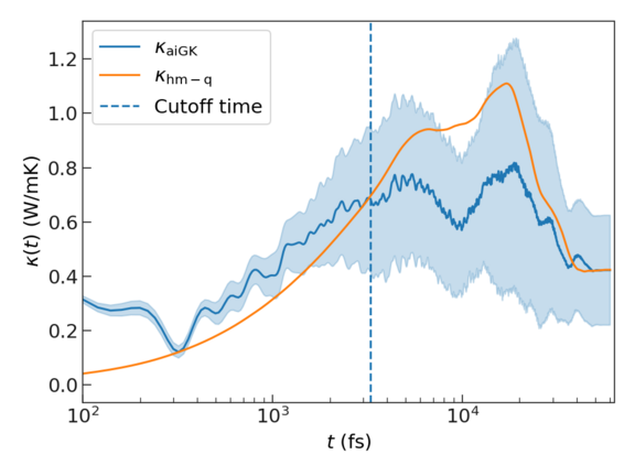
The blue line is the ab initio Green-Kubo calculated heat flux, with the filled area shows the standard deviation across different directions. The harmonic heat flux, \(\boldsymbol{J}_{\rm{hm-q}}(t)\) is given by the orange line, and the vertical line shows the cutoff time determined by the first dip method.
The plot greenkubo_interpolation_lifetimes.pdf shows the phonon mode energy auto-correlation function and is shown below.
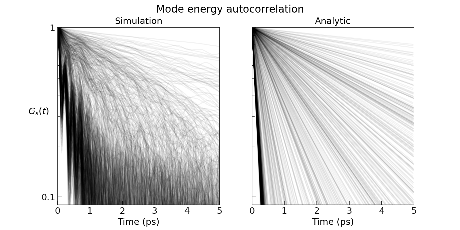
We borrow the assumption from the perturbation theory, the leading contribution to the phonon decay can be approximated via,
Under this approximation, the integral can be performed analytically based on the early decay of the correlation function, hence allowing to capture also those long-lived, long-wavelength modes that are not guaranteed to be accessible via brute-force integration on the simulation timescales accessible in aiMD simulations.
The plot greenkubo_interpolation_fit.pdf shows the interpolation and extrapolation results and is shown below.
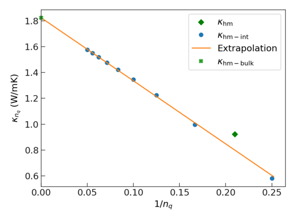
This plot shows how it is possible to extrapolate to an infinite system size, i.e., to the bulk limit of the thermal conductivity. The x axis is given in terms of \(1/n_{q}\), where \(n_{q}\) is the number of q points.
- The green diamond shows the results one obtains without interpolation. To this end, the ab initio MD data is mapped to reciprocal space and the thermal conductivity is evaluated using the BTE. Note that the employed supercell corresponds to a q-point density in reciprocal space of \(1/n_q \approx 0.22\).
- The blue dots show results obtained by first mapping the ab initio MD data to reciprocal space and then interpolating the data to denser q-point grids (smaller values of \(n_q\)).
- The orange line shows a linear fit of the interpolated data that can be used to extrapolate to infinite size (where \(1/n_q\) → 0). Hence the thermal conductivity at infinite q grid density \(\kappa_{\rm bm-bulk}\) is the intercept of the linear fit.
The finite-size correction \(\Delta \kappa\) is calculated by,
As the output information shows, the thermal conductivity after correction is \(1.696 \pm 0.274\) W/mK.
Convergence of simulation time#
Convergence with respect to simulation time is important for a reliable calculation from the aiGK method.
The --shorten argument in vibes output gk is provided to test the convergence.
For our example of nve.1/trajectroy.nc, CuI with simulation time of \(60 {\rm ps}\), the following command
can be used for performing Green-Kubo calculation on a shortened trajectory with simulation time \(0.8 \times t_{0}\), with \(t_0\) being the simulation time of the full trajectory.
A bash script and a python script is provided in
Tutorial/greenkubo/3_greenkubo/solutions
for helping with the postprocessing and plotting of the simulation time convergence.
You can copy both scripts to the result directory, for example nve.1, and run the following command
The produced plot simulation_time_convergence.pdf will show the thermal conductivity
as a function of simulation time.
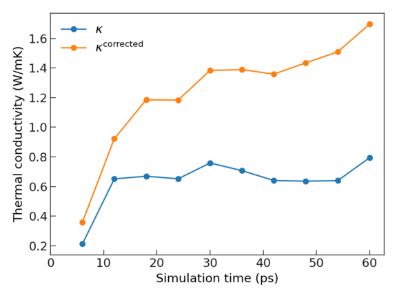
The blue curve shows the thermal conductivity from the bare Green-Kubo results, and the orange curve shows the finite-size corrected results.
Ensemble average#
In practice, we need to evaluate the thermal conductivity from multiple MD trajectories in order to have an appropriate ensemble average. For sampling the phase space, the configurations can be chosen from an NVT MD simulation.
For NVT MD simulation, geometry.in.supercell and geometry.in.primitive follows the same
as introduced in Setting up ab initio MD.
The initial step geometry.in can be generated by random displacement with the kinetic
energy at target temperature \(300\) K, with the following command:
Here are an example of md.in to perform NVT calculations,
Example of md.in
[files]
geometry:                      geometry.in
primitive:                     geometry.in.primitive
supercell:                     geometry.in.supercell


[calculator]
name:                          aims
socketio:                      true

[calculator.parameters]
xc:                            pbesol
compute_forces:                true
compute_analytical_stress:     true
compute_heat_flux:             true

[calculator.kpoints]
density:                       2

[calculator.basissets]
Cu:                            light
I:                             light

[slurm]
name:                          nvt
tag:                           vibes
mail_type:                     none
mail_address:                  your@mail.com
nodes:                         2
cores:                         40
queue:                         general
timeout:                       600


[md]
driver:                        Langevin
timestep:                      5
maxsteps:                      2000
compute_stresses:              2
workdir:                       md

[md.kwargs]
temperature:                   300
friction:                      0.02
logfile:                       md.log


[restart]
command = sbatch submit.sh
Here we are using Langevin thermostat with friction parameters of \(0.02\) and temperature of \(300\) K. The full tutorial on NVT MD simulation can be found in ab initio MD in FHI-vibes tutorial.
An example NVT trajectory can be found here (nvt.1/trajectory.nc) You can then use the command like
to pick, for example, configuration No. \(1500\) from the NVT trajectory as a starting point for NVE calculation.
Another NVE trajectory is provided here (nve.3/trajectory.nc). The thermal conductivity with finite size correction from this trajectory is \(2.120 \pm 0.432\) W/mK. The ensemble average from these two trajectories is \(1.908 \pm 0.270\) W/mK, which is very close to the CRC Handbook reference of \(1.68\) W/mK, much better than the result from BTE of \(5.918\) W/mK.
Strong anharmonicity#
The analysis of the aiMD dynamics reveals strongly anharmonic effects in this CuI system. This is evident from the time evolution of the anharmonicity measure, \(\sigma^{A}(t)\), as shown in the figure below.
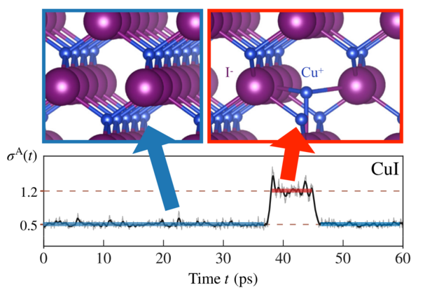
This measure, introduced in Ref 3, quantifies the deviation between the actual potential-energy surface (PES) and its harmonic approximation, and it would be zero in an ideal harmonic material.
The constant value of 0.5 indicates already some significant anharmonicity in the system, and there is also a sharp increase in \(\sigma^{A}(t)\) from 0.5 to 1.2 indicating extreme anharmonicity in this period, where the harmonic approximation will surely fail to accurately describe the dynamics. In this time period of several picoseconds, a metastable Frenkel defect forms. The upper part of the figure illustrates this process, where a Cu cation migrates to an interstitial site along the \((\bar{1}11)\) direction and oscillates around the metastable defect geometry. Eventually, it returns to the zinc-blende equilibrium configuration, where \(\sigma^{A}(t)\) reverts to approximately 0.5.
This transient defect formation can be interpreted as a localized precursor to the superionic \(\beta\)-phase of CuI. This phase, characterized by a substantial defect concentration exceeding 10%, becomes stable only at significantly higher temperatures (above 643 K).
Solutions#
You find all the solution to all the above exercises by clicking on the button below.