Thermal Transport in Strongly Anharmonic CuI#
Estimated total CPU time: < 5 min when using 70 cores or more
Info
This is a concise tutorial created for the FHI-aims webinar series given in December 2024. It introduces participants to heat-transport theory and covers the most important aspects, but it is far from exhaustive. For learning more about these kinds of calculations, we strongly recommend to also check the longer, full-fledged tutorials in later sections, which provide more detailed explanations and exercises.
Prerequisites#
- Installed (parallel) version of FHI-aims, version
240920or newer. - Installed version of FHI-vibes, version
v1.1.0or newer. - Compute resources of about 70 cores.
What makes CuI an intriguing testcase?#
At low temperatures, the nuclear motion in most materials can be approximately described with relatively simple models, namely with decoupled harmonic oscillators that capture how atoms vibrate around their equilibrium position. Obviously, this is an approximation and anharmonic effects beyond the harmonic approximation can influence the dynamics as well. For instance, heat transport is largely influenced by the strength of anharmonic effects.
When atoms vibrate in a crystal, their movements create wave-like patterns we call phonons, as if the atoms would be connected by springs following Hooke's law. In a ficticious, perfectly harmonic crystal, phonons are decoupled from each other and hence travel forever without scattering, resulting in an infinite thermal conductivity. In real materials, however, phonons interact with each other through anharmonic effects. Accordingly, phonons have finite lifetimes and materials have finite thermal conductivities.
The Boltzmann Transport Equation (BTE) is one of the most common methods for modeling heat transport from first principles. As discussed below, it is based on treating phonon-phonon interactions as small perturbations. While this works well for many materials, it has limitations - particularly for strongly anharmonic systems. In that case, non-perturbative methods such as the Green-Kubo approach need to be used to obtain accurate results, as also discussed below.
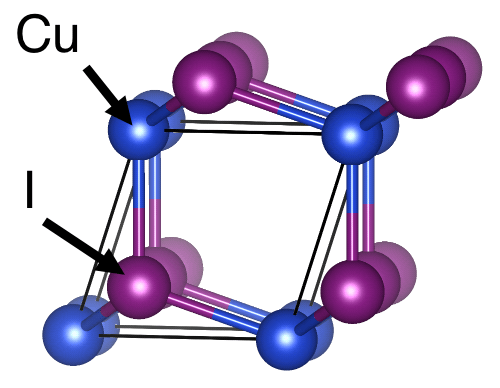
Typically, anharmonic effects are stronger at higher temperatures and/or in complex compounds. In this regard, copper iodide (CuI) constitutes an interesting test case for studying, explaining, and understanding heat transport. Despite crystallizing in a simple, zinc-blende structure (space group \(\rm F\bar{4}3m\)), the dynamics of copper iodide (CuI) are affected by strong anharmonic effects already at room temperature. This allows us to discuss and quantify how such strongly anharmonic effects influence heat transport. For a more in-depth coverage of these topics, please also refer to the publications45 that this tutorial is based on.
In CuI, the copper atoms show large deviations from the harmonic behavior even at room temperature. These are not just small perturbations - they are significant enough to fundamentally change how heat moves through the crystal. What makes this case particularly interesting from a physics perspective is that these anharmonic effects are possible precursors to a phase transition. Above 643 K, CuI transforms into a superionic conductor, where copper ions become highly mobile within the crystal lattice 6. But even at room temperature, we can see signatures of this transition in the copper atoms' dynamics. The atoms show large-amplitude motions that occasionally result in temporary defect structures - a phenomenon that is impossible to capture with harmonic or weakly anharmonic approximations.
In this tutorial, we will explore how to properly calculate thermal transport in such a strongly anharmonic system. We will start with standard harmonic phonon calculations to establish a baseline and understand the system's basic vibrational properties. Then, we will see how to perform perturbative BTE calculations and non-perturbative ab initio Green-Kubo calculations. Through this progression, you are going to learn how, when, and why to use these different theoretical frameworks.
Phonons: Harmonic Vibrations#
Info
This is only a short introduction to the basic concepts of phonon theory needed for this tutorial. A more extensive introduction can be found on this page.
Formally, phonons can be described by the harmonic approximation. To this end, we expand the potential-energy surface \(E({\boldsymbol{R}})\) around the energetic minimum \(\boldsymbol{R}^0\) in terms of displacements from equilibrium up to second order and neglect all higher-order (anharmonic) terms. Accordingly, the first non-trivial and non-vanishing term in this approximation is given by the Hessian \(\boldsymbol{\Phi}_{IJ}\).
In this tutorial we use the finite displacement method to calculate the Hessian from first principles. For this purpose, we slightly displace one atom from its equilibrium position (by a small displacement \(\varepsilon\)) and calculate the forces \(\boldsymbol{F}_J\) on all other atoms. Mathematically, this yields:
By repeating this procedure, we can approximately map out how atoms interact with each other. In simple, high-symmetry crystals like CuI, we can additionally exploit crystal symmetry. By this means, we only need to displace few atoms and not all of them to construct the Hessian. Once the Hessian is calculated, all phonon-related properties can be derived from it.
Phonon calculations with FHI-vibes and phonopy#
Warning
In the following exercises, the computational settings, in particular the reciprocal space grid (tag k_grid), the basis set and supercell sizes, have been chosen to allow a rapid computation of the exercises. Although the qualitative trends already hold with the present settings, the reciprocal space grid, the basis set, and the supercells would all have to be converged with much more care for real production calculations.
Now that we understand the basic theory, we now see how to actually perform these calculations using FHI-vibes. FHI-vibes connects the FHI-aims software (which handles our quantum mechanical calculations) with phonopy 2 (which handles the setup and analysis of the phonon calculations). Please note that phonopy makes extensive use of symmetry analysis 3, which allows to reduce numerical noise and to speed up the calculations considerably.
We start by creating a new working folder called CuI_phonons and then navigating to that folder with
In here we need to create 2 files:
geometry.in- this contains the primitive cell structure of CuIphonopy.in- this contains our calculation settings forFHI-vibes
The geometry.in file needs to contain the relaxed primitive structure of CuI. Create the file geometry.in and copy in the following block into the file:
lattice_vector 0.0000000004000000 3.0070256877000001 3.0070256877000001
lattice_vector 3.0070256877000001 0.0000000004000000 3.0070256877000001
lattice_vector 3.0070256877000001 3.0070256877000001 0.0000000004000000
atom 0.0000000000000000 0.0000000000000000 0.0000000000000000 Cu
atom 1.5035128439500001 1.5035128439500001 1.5035128439500001 I
Next, create another file called phonopy.in and fill it with this content:
[files]
geometry:                      geometry.in

[calculator]
name:                          aims
socketio:                      true

[calculator.parameters]
xc:                           pbesol
compute_forces:               true

[calculator.kpoints]
density:                      2

[calculator.basissets]
Cu:                           light
I:                            light

[phonopy]
supercell_matrix:             [-2,  2,  2,  2, -2,  2,  2,  2, -2]
displacement:                 0.01
is_diagonal:                  False
is_plusminus:                 auto
symprec:                      1e-05
q_mesh:                       [45, 45, 45]
workdir:                      phonopy
An explanation of all parameters is given in the FHI-vibes documentation. The most important parameter here is the supercell_matrix, which determines the size of our calculation cell (as described in the FHI-vibes tutorials). Formally, this determines the size of the Hessian matrix; from a physics point of view, this limits the range of interactions that are considered. Accordingly, choosing this size properly is crucial - too small supercells yield unconverged, inaccurate results, while too large supercells become unnecessarily costly. Here, we use a cubic supercell with 64 atoms for CuI, which is not converged but already correctly captures the trends for the phonon band structure. FHI-vibes has a utility function that can help you find cubic-like supercells of different sizes as explained in more detail here.
Once your files are ready, you can submit the calculation to the compute cluster with:
Example for the submission script on the webinar cluster
#!/bin/bash -l
# Standard output and error:
#SBATCH -o ./slurm.stdout
#SBATCH -e ./slurm.stderr
# Initial working directory:
# Standard output and error:
#SBATCH -o ./slurm.stdout
#SBATCH -e ./slurm.stderr
# Initial working directory:
#SBATCH -D ./
# Job Name:
#SBATCH -J FHI-aims
# Number of nodes and MPI tasks per node:
#SBATCH --nodes=1
# HPC7a
#SBATCH --tasks-per-node=192
#
# Wall clock limit:
#SBATCH --time=00:05:00

module purge
module load fhi-aims vibes

date
vibes run phonopy
The calculation should take around a minute on the provided resources. FHI-vibes will create a series of displaced structures, calculate the acting forces using FHI-aims, and collect all the results in a file called trajectory.son in the phonopy directory.
To assemble the Hessian, compute the phonon properties, and analyze the results, run:
This command calculates various phonon properties (frequencies, dispersion relations, density of states) and saves them in the phonopy/output directory. You will find a plot of the phonon band structure and density of states in bandstructure_dos.pdf.
You can copy the results and the full output folder to your local machine using the scp command, by running the following from your local machine:
If everything worked correctly, you should get a plot that looks like this:
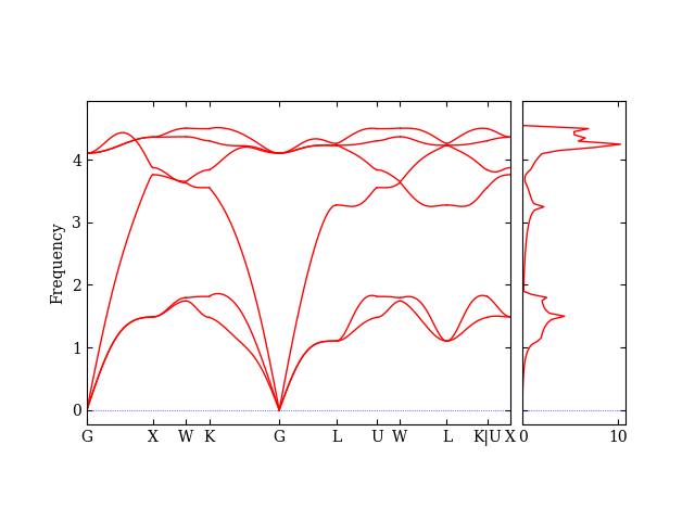
This plot shows the phonon frequencies (y-axis) along different directions in the Brillouin zone (x-axis), along with the phonon density of states (right panel). The absence of negative frequencies indicates that our structure is stable.
Thermal Conductivity via the Boltzmann Transport Equation#
The Boltzmann Transport Equation (BTE) is one of the most common approaches to calculate thermal conductivities from first principles. It is based on the harmonic approximation, which is used to model the dynamics of the nuclei. In comparison, anharmonic effects are assumed to be small, so that they can be treated perturbatively, without explicitly considering anharmonic effects in the dynamics.
In the BTE approach, the thermal conductivity can be written as:
Here, \(c_{\lambda}\) is the heat capacity of a phonon mode, \(\boldsymbol{v}_{\lambda}\) is its group velocity, and \(\tau_{\lambda}\) its lifetime. The sum runs over all phonon modes \(\lambda\). While heat capacity and group velocity can be obtained in the harmonic approximation, phonon lifetimes require to consider anharmonic effects. Here, we only account for the lowest order of anharmonic effects by extending the expansion of the potential-energy surface by one term, the third-order term. Essentially, these third-order force constants describe how the force on one atom changes when two other atoms are displaced from their equilibrium positions. All other, higher-order anharmonic effects are neglected.
More details on the theoretical background of BTE calculations can be found here.
BTE calculation with FHI-vibes#
To run a thermal conductivity calculation using the BTE approach with FHI-vibes and phono3py, create a new working directory:
Like before, we need two files:
geometry.in- the same primitive cell structure we used for computing the phononsphono3py.in- settings for our thermal transport calculation
Create the geometry.in file with the same content as before by copying the file from your old phonon folder
and then create the phono3py.in file:
[files]
geometry:                     geometry.in

[calculator]
name:                         aims
socketio:                     true

[calculator.parameters]
xc:                           pbesol
compute_forces:               true

[calculator.kpoints]
density:                      2

[calculator.basissets]
Cu:                           light
I:                            light

[phono3py]
supercell_matrix:             [-3,  3,  3,  3, -3,  3,  3,  3, -3]
cutoff_pair_distance:         6.0
workdir:                      phono3py
Note
Notice that we are now using a larger supercell_matrix, which results in a 64-atom cell. Unlike our earlier phonon calculations, we are using a converged supercell size here since we are providing the results.
This calculation will generate 102 displaced structures for CuI. Processing all these displacements takes considerably longer than a simple phonon calculation. For this tutorial, we provide pre-calculated results on the compute resources in ~/CuI_output/CuI_thermal_BTE that you can copy to your local folder to continue with the tutorial.
Copy the results to this folder with:
To process the results, run
This will take a couple of minutes.Finally, calculate the thermal conductivity with
Note
If you find the postprocessing is very slow, maybe you are running on a single core.
You could try export OMP_NUM_THREADS=<number_of_cores> to use more threads on the local machine and accelerate the phono3py post-processing.
The --mesh parameter controls the \(q\)-mesh density on which the phonon-phonon scattering events are calculated. The thermal conductivity and many related properties are written into the file kappa-m666.hdf5.
Output of phono3py-load phono3py_params.yaml --mesh 6 6 6 --br
...
----------- Thermal conductivity (W/m-k) with tetrahedron method -----------
#  T(K)        xx         yy         zz         yz         xz         xy
   0.0       0.000      0.000      0.000      0.000      0.000      0.000
  10.0    3374.939   3374.939   3374.939     -0.000     -0.000     -0.000
  20.0     563.452    563.452    563.452     -0.000     -0.000     -0.000
  30.0     158.345    158.345    158.345     -0.000     -0.000     -0.000
  40.0      72.640     72.640     72.640     -0.000     -0.000     -0.000
  50.0      44.459     44.459     44.459     -0.000     -0.000     -0.000
  60.0      31.723     31.723     31.723     -0.000     -0.000     -0.000
  70.0      24.695     24.695     24.695     -0.000     -0.000     -0.000
  80.0      20.284     20.284     20.284     -0.000     -0.000     -0.000
  90.0      17.261     17.261     17.261     -0.000     -0.000     -0.000
 100.0      15.057     15.057     15.057     -0.000     -0.000     -0.000
 110.0      13.376     13.376     13.376     -0.000     -0.000     -0.000
 120.0      12.048     12.048     12.048     -0.000     -0.000     -0.000
 130.0      10.970     10.970     10.970     -0.000     -0.000     -0.000
 140.0      10.077     10.077     10.077     -0.000     -0.000     -0.000
 150.0       9.323      9.323      9.323     -0.000     -0.000     -0.000
 160.0       8.679      8.679      8.679     -0.000     -0.000     -0.000
 170.0       8.120      8.120      8.120     -0.000     -0.000     -0.000
 180.0       7.631      7.631      7.631     -0.000     -0.000     -0.000
 190.0       7.199      7.199      7.199     -0.000     -0.000     -0.000
 200.0       6.815      6.815      6.815     -0.000     -0.000     -0.000
 210.0       6.471      6.471      6.471     -0.000     -0.000     -0.000
 220.0       6.160      6.160      6.160     -0.000     -0.000     -0.000
 230.0       5.879      5.879      5.879     -0.000     -0.000     -0.000
 240.0       5.622      5.622      5.622     -0.000     -0.000     -0.000
 250.0       5.388      5.388      5.388     -0.000     -0.000     -0.000
 260.0       5.172      5.172      5.172     -0.000     -0.000     -0.000
 270.0       4.974      4.974      4.974     -0.000     -0.000     -0.000
 280.0       4.790      4.790      4.790     -0.000     -0.000     -0.000
 290.0       4.619      4.619      4.619     -0.000     -0.000     -0.000
 300.0       4.461      4.461      4.461     -0.000     -0.000     -0.000
 310.0       4.313      4.313      4.313     -0.000     -0.000     -0.000
 320.0       4.175      4.175      4.175     -0.000     -0.000     -0.000
 330.0       4.045      4.045      4.045     -0.000     -0.000     -0.000
 340.0       3.923      3.923      3.923     -0.000     -0.000     -0.000
 350.0       3.809      3.809      3.809     -0.000     -0.000     -0.000
 360.0       3.701      3.701      3.701     -0.000     -0.000     -0.000
 370.0       3.599      3.599      3.599     -0.000     -0.000     -0.000
 380.0       3.502      3.502      3.502     -0.000     -0.000     -0.000
 390.0       3.411      3.411      3.411     -0.000     -0.000     -0.000
 400.0       3.324      3.324      3.324     -0.000     -0.000     -0.000
 410.0       3.242      3.242      3.242     -0.000     -0.000     -0.000
 420.0       3.164      3.164      3.164     -0.000     -0.000     -0.000
 430.0       3.089      3.089      3.089     -0.000     -0.000     -0.000
 440.0       3.018      3.018      3.018     -0.000     -0.000     -0.000
 450.0       2.950      2.950      2.950     -0.000     -0.000     -0.000
 460.0       2.885      2.885      2.885     -0.000     -0.000     -0.000
 470.0       2.823      2.823      2.823     -0.000     -0.000     -0.000
 480.0       2.763      2.763      2.763     -0.000     -0.000     -0.000
 490.0       2.706      2.706      2.706     -0.000     -0.000     -0.000
 500.0       2.652      2.652      2.652     -0.000     -0.000     -0.000
 510.0       2.599      2.599      2.599     -0.000     -0.000     -0.000
 520.0       2.549      2.549      2.549     -0.000     -0.000     -0.000
 530.0       2.500      2.500      2.500     -0.000     -0.000     -0.000
 540.0       2.453      2.453      2.453     -0.000     -0.000     -0.000
 550.0       2.408      2.408      2.408     -0.000     -0.000     -0.000
 560.0       2.365      2.365      2.365     -0.000     -0.000     -0.000
 570.0       2.323      2.323      2.323     -0.000     -0.000     -0.000
 580.0       2.283      2.283      2.283     -0.000     -0.000     -0.000
 590.0       2.244      2.244      2.244     -0.000     -0.000     -0.000
 600.0       2.206      2.206      2.206     -0.000     -0.000     -0.000
 610.0       2.170      2.170      2.170     -0.000     -0.000     -0.000
 620.0       2.135      2.135      2.135     -0.000     -0.000     -0.000
 630.0       2.100      2.100      2.100     -0.000     -0.000     -0.000
 640.0       2.067      2.067      2.067     -0.000     -0.000     -0.000
 650.0       2.035      2.035      2.035     -0.000     -0.000     -0.000
 660.0       2.004      2.004      2.004     -0.000     -0.000     -0.000
 670.0       1.974      1.974      1.974     -0.000     -0.000     -0.000
 680.0       1.945      1.945      1.945     -0.000     -0.000     -0.000
 690.0       1.917      1.917      1.917     -0.000     -0.000     -0.000
 700.0       1.889      1.889      1.889     -0.000     -0.000     -0.000
 710.0       1.862      1.862      1.862     -0.000     -0.000     -0.000
 720.0       1.836      1.836      1.836     -0.000     -0.000     -0.000
 730.0       1.811      1.811      1.811     -0.000     -0.000     -0.000
 740.0       1.787      1.787      1.787     -0.000     -0.000     -0.000
 750.0       1.763      1.763      1.763     -0.000     -0.000     -0.000
 760.0       1.739      1.739      1.739     -0.000     -0.000     -0.000
 770.0       1.717      1.717      1.717     -0.000     -0.000     -0.000
 780.0       1.695      1.695      1.695     -0.000     -0.000     -0.000
 790.0       1.673      1.673      1.673     -0.000     -0.000     -0.000
 800.0       1.652      1.652      1.652     -0.000     -0.000     -0.000
 810.0       1.632      1.632      1.632     -0.000     -0.000     -0.000
 820.0       1.612      1.612      1.612     -0.000     -0.000     -0.000
 830.0       1.592      1.592      1.592     -0.000     -0.000     -0.000
 840.0       1.573      1.573      1.573     -0.000     -0.000     -0.000
 850.0       1.554      1.554      1.554     -0.000     -0.000     -0.000
 860.0       1.536      1.536      1.536     -0.000     -0.000     -0.000
 870.0       1.519      1.519      1.519     -0.000     -0.000     -0.000
 880.0       1.501      1.501      1.501     -0.000     -0.000     -0.000
 890.0       1.484      1.484      1.484     -0.000     -0.000     -0.000
 900.0       1.468      1.468      1.468     -0.000     -0.000     -0.000
 910.0       1.452      1.452      1.452     -0.000     -0.000     -0.000
 920.0       1.436      1.436      1.436     -0.000     -0.000     -0.000
 930.0       1.420      1.420      1.420     -0.000     -0.000     -0.000
 940.0       1.405      1.405      1.405     -0.000     -0.000     -0.000
 950.0       1.390      1.390      1.390     -0.000     -0.000     -0.000
 960.0       1.376      1.376      1.376     -0.000     -0.000     -0.000
 970.0       1.362      1.362      1.362     -0.000     -0.000     -0.000
 980.0       1.348      1.348      1.348     -0.000     -0.000     -0.000
 990.0       1.334      1.334      1.334     -0.000     -0.000     -0.000
1000.0       1.321      1.321      1.321     -0.000     -0.000     -0.000
Thermal conductivity related properties were written into
"kappa-m666.hdf5".
...
We find that the thermal conductivity at 300 K is 4.46 W/mK at this \(q\) mesh density. For production calculations, you should converge the mesh size. For example, with a \(20 \times 20 \times 20\) mesh, we get a converged, room-temperature thermal conductivity of 5.92 W/mK.
Important
In comparison to our result, the experimental thermal conductivity of CuI is reported to be much lower, around 1.68 W/mK 7. Our BTE calculation overestimates this value by more than 350%. We will discuss the reasons for this disagreement in the following section.
Thermal Conductivity via the Green-Kubo Approach#
While the BTE method is based on the harmonic approximation and treats all anharmonicity perturbatively, the Green-Kubo approach is based on explicit molecular dynamics (MD) on the full, non-approximated potential-energy surface. This allows to accurately capture all orders of anharmonic effects in a non-pertubative fashion. The details on the theory and implementation can be found in Ref.[^Knoop2020,^Knoop2023a,^Knoop2023b].
The key idea is simple but powerful: if we track the heat current in our MD simulation, its fluctuations tell us about thermal conductivity. This is a general principle called the fluctuation-dissipation theorem, which relates fluctuations in thermal equilibrium to transport under non-equilibrium conditions. For the thermal conductivity, the resulting Green-Kubo formula reads:
Here, \(\boldsymbol{J}(t)\) is the heat current at time \(t\) and we are computing its time-auto-correlation function in thermodynamic equilibrium. In simple terms, we hence measure how long heat-flow fluctuations persist - the longer they persist, the higher the thermal conductivity.
Note
Running ab initio MD in extended supercells for tens of picoseconds takes considerable computer time, much more than available within a short one-hour tutorial. For detailed instructions on setting up and running MD calculations with FHI-vibes in the context of Green-Kubo simulations, please refer to the longer tutorial. In this tutorial, we provide pre-calculated trajectories in the FHI-vibes format in the folders ~/CuI_outputs/CuI_GK/nve.1/trajectory.nc and ~/CuI_outputs/CuI_GK/nve.2/trajectory.nc for you to analyze. These trajectories stem from Ref. 4, and you can download the full trajectories to your local machine (~1 GB filesize) from here.
Create a new working folder with
Copy the pre-calculated trajectories to your folder with:
To analyze the results, first check the MD trajectory provided in the directory nve.1:
Output of vibes info md trajectory.nc
Dataset summary for trajectory.nc:

[info]         Summarize Displacements
Avg. Displacement:             0.22949 AA
Max. Displacement:             2.8811 AA
Avg. Displacement [Cu]:        0.26255 AA
Avg. Displacement [I]:         0.19642 AA

[info]         Summarize Forces
Avg. Force:                    1.1855e-19 eV/AA
Std. Force:                    0.35737 eV/AA
Std. Force [Cu]:               0.30548 eV/AA
Std. Force [I]:                0.40264 eV/AA

[info]         Summarize Temperature
Simulation time:                 60.000 ps (12001 steps)
Temperature:                       310.237 +/-      12.7020 K
Temperature (first 1/2):           311.385 +/-      12.4513 K
Temperature (last  1/2):           309.089 +/-      12.8466 K
Temperature drift:                  -0.05838 K/ps

[info]         Summarize Potential Pressure
Simulation time:                 60.000 ps (3062 of 12001 steps)
Pressure:                          0.061724 +/-   0.056299 GPa
Pressure (last 1/2):               0.046461 +/-   0.055929 GPa
Pressure (last 1/2):               0.000290 +/-   0.000349 eV/AA**3
[info]         Summarize Total Pressure (Kinetic + Potential)
Simulation time:                 60.000 ps (3062 of 12001 steps)
Pressure:                          0.219238 +/-   0.054823 GPa
Pressure (last 1/2):               0.203353 +/-   0.054621 GPa
Pressure (last 1/2):               0.001269 +/-   0.000341 eV/AA**3

[info]         Drift
Mean abs. Momentum:            [1.8597e-13 1.6907e-13 1.5333e-13] AA/fs
Energy drift:                  -1.02111e-05  eV / timestep
Energy change after 100ps:     -2.04222e-01  eV
Energy change after 100ps:     -9.45472e-01  meV / atom (n=216)
This will output a short summary for the trajectory, including average and maximum atomic displacements, forces, system temperature and pressure, as well as the energy drift. All of which are important quantities to judge the quality of the trajectory.
Next, calculate the thermal conductivity:
Output from vibes output gk trajectory.nc
Run aiGK output workflows for trajectory.nc
[GreenKubo]    Compute Prefactor:
[GreenKubo]    .. Volume:           5873.07  AA^3
[GreenKubo]    .. Temperature:       310.24  K
[GreenKubo]    -> Prefactor:      1.135e+03  W/mK / (eV/AA^2/fs)
[GreenKubo]    Estimate filter window size
[GreenKubo]    .. lowest vibrational frequency: 0.8364 THz
[GreenKubo]    .. corresponding window size:    1195.5435 fs
[GreenKubo]    .. window multiplicator used:    1.0000 fs
[filter]       Apply Savitzky-Golay filter with {'window_length': 61, 'polyorder': 1}
[GreenKubo]    Cutoff times (fs):
[GreenKubo]    [[5360.    0.    0.]
[GreenKubo]     [   0. 1480.  940.]
[GreenKubo]     [   0.  420. 2960.]]
[GreenKubo]    Kappa is:       0.795 +/- 0.274 W/mK
[GreenKubo]    Kappa^ab is:
[GreenKubo]    [[ 1.423e+00 -1.168e-03 -1.080e-03]
[GreenKubo]     [-1.387e-04  2.769e-01  1.053e-02]
[GreenKubo]     [-1.092e-03  1.441e-02  6.843e-01]]
As you can see from the output, several settings such as the filter window size are chosen automatically based on the trajectory data. Based on these, the thermal conductivity is computed as an average over the trace and as the full 3x3 matrix.
We can also visualize the result. First, we look at the Green-Kubo analysis:
Copy the resulting plots to a local folder with
and inspect the figure greenkubo_summary.pdf.
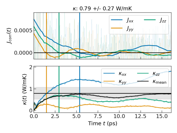
The plot shows two important things:
-
Top panel: The heat flux auto-correlation function. The thin lines show the raw data, while the thick lines show the post-processed data, for which the noise and fluctuations that do not contribute to the thermal conductivity have been removed. The vertical lines indicate the earliest occurrence of the auto-correlation functions crossing the x-axis. We assume that the auto-correlation function is trustworthy up to this "first dip". Accordingly, the thermal conductivities reported in the output are obtained by integrating up to this time.
-
Bottom panel: The running integral of the above auto-correlation functions that yields the thermal conductivity. Each colored line represents a different direction (xx, yy, zz), the black line their mean, and the shaded area the associated standard deviation.
Since CuI has cubic symmetry (space group F4̄3m), the thermal conductivity should be the same along all Cartesian axis (\(\kappa_{xx} = \kappa_{yy} = \kappa_{zz}\)). The differences observed in the simulation stem from the fact that only a small portion of phase space can be captured in such short ab initio MD simulations. For this reason, it is recommended to always run multiple trajectories with different initial conditions, until the respective ensemble average yields statistically converged results.
The above procedure allows to correct for the finite-time addressable in ab initio MD simulations. Similarly, ab initio MD is typically run in relatively small supercells with a small number of atoms. Accordingly, potentially important long-wavelength vibrations are neglected in the raw ab initio MD data. One can correct for these finite-size effects by mapping the simulations to frequency- and reciprocal-space. In this space, a finite-size extrapolation corresponds to a Brillouin zone interpolation, which is numerically advantageous. This is achieved by running:
Again, copy the resulting plots to your local machine with
and inspect greenkubo_interpolation_fit.pdf.
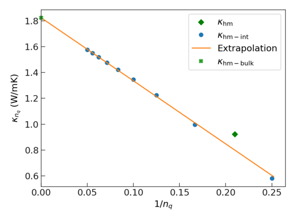
This plot shows how it is possible to extrapolate to an infinite system size, i.e., to the bulk limit of the thermal conductivity:
- The green diamond shows the results one obtains without interpolation. To this end, the ab initio MD data is mapped to reciprocal space and the thermal conductivity is evaluated using the BTE. Note that the employed supercell corresponds to a q-point density in reciprocal space of \(1/n_q \approx 0.22\).
- The blue dots show results obtained by first mapping the ab initio MD data to reciprocal space and then interpolating the data to denser q-point grids (smaller values of \(n_q\)).
- The orange line shows a linear fit of the interpolated data that can be used to extrapolate to infinite size (where \(1/n_q\) → 0).
The finite-size correction \(\Delta\kappa\), which has to be added on top of our finite-cell results discussed above, is then calculated as the difference between the extrapolated value (\(\kappa_{\rm hm-bulk}\)) and our simulation cell value (\(\kappa_{\rm hm}\)):
After the correction, we obtain a value of 1.696 ± 0.274 W/mK. To improve our statistics, we can average results from multiple trajectories. For instance, the second trajectory provided in ~/CuI_outputs/CuI_GK/nve.2/trajectory.nc yields a value of 2.120 ± 0.432 W/mK. The ensemble average of both trajectories is 1.908 ± 0.270 W/mK. Feel free to analyse the trajectory in folder nve.2 by yourself!
Compared to the BTE approach discussed before, the Green-Kubo calculations yield a much lower thermal conductivity (5.9 vs. 1.9 W/mK) that also lies closer to the experimental value of 1.7 W/mK. The reason for this failure of the BTE lies in the strongly anharmonic nature of CuI, which we can actually see in our trajectories. This plot from Ref. 4 reveals the complex dynamics in this system:
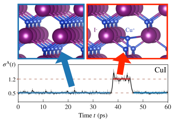
The bottom panel tracks the anharmonicity measure \(\sigma^A(t)\) 1 throughout the simulation. A value of 0 corresponds to a perfectly harmonic system. In CuI, this measure stays around 0.5 for long times, indicating that 50% of the interactions stem from anharmonic effects. This already indicates strong anharmonic effects. On top of that, we observe that the anharmonicity can jump to even higher values, for instance between 35 to 48 ps. Here, the harmonic approximation breaks down completely. The top panel reveals what is happening during these anharmonicity jumps: a copper atom temporarily leaves its normal lattice site and moves to an interstitial position, forming a Frenkel defect, before eventually returning to its original position. It now becomes clear why the BTE approach overestimates the conductivity and underestimates the anharmonicity. By treating the anharmonicity as a small perturbation, it simply cannot capture the short-lived formation of such defect structures. Accurately capturing these effects via the Green-Kubo approach is hence crucial for accurately predicting thermal properties in strongly anharmonic materials like CuI.
-
F. Knoop, T. A. Purcell, M. Scheffler, and C. Carbogno, Phys. Rev. Mater. 4.8 083809 (2020). ↩
-
Atsushi Togo and Isao Tanaka, Scr. Mater., 108, 1-5 (2015). ↩
-
K. Parlinski, Z. Q. Li, and Y. Kawazoe, Phys. Rev. Lett. 78, 4063 (1997). ↩
-
F. Knoop, T. A. Purcell, M. Scheffler, and C. Carbogno, Phys. Rev. Lett. 130, 236301 (2023). ↩↩↩
-
F. Knoop, M. Scheffler, and C. Carbogno, Phys. Rev. B. 107, 224304 (2023). ↩
-
D. A. Keen and S. Hull, J. Phys. Condens. Matter 7, 5793 (1995). ↩
-
CRC Handbook of Chemistry and Physics, David R. Lide, Ed. 79th Edition, CRC Press, Boca Raton, FL, 1998. ↩